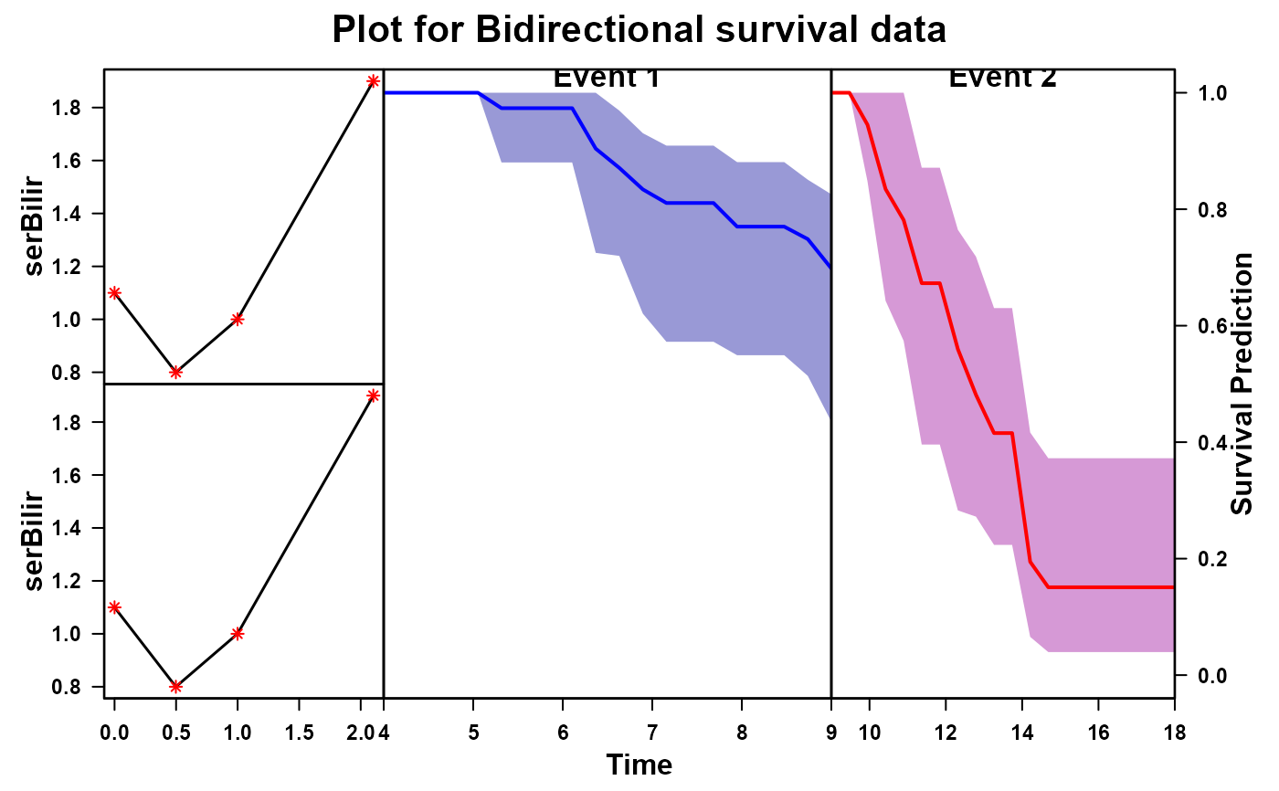
Prediction plot from jmcsB()

Prediction plot from jmcsB()

Usage

# S3 method for jmcsB
plot(x, y, ...)

Arguments

x

fitted model object

y

newdata longitudinal

...

other

Value

Returns prediction plot for the newdata using the model fitted through jmcsB()

Note

In the example code we use newdata as the data for ID 2 in the PBC2 dataset, it has follow up information till 8.832. Now suppose we want to look at the survival of ID 2 under joint model 1 after time 4 and for joint model 2 after time 9. For that we created the newdata as if the individual is followed till for a time period less than min(4,9).

Examples

 # \donttest{
 library(JMbayes2)
 library(FastJM)
  st_pbcid<-function(){
  new_pbcid<-pbc2.id
  new_pbcid$time_2<-rexp(n=nrow(pbc2.id),1/10)
  cen_time<-runif(nrow(pbc2.id),min(new_pbcid$time_2),max(new_pbcid$time_2))
  status_2<-ifelse(new_pbcid$time_2<cen_time,1,0)
  new_pbcid$status_2<-status_2
  new_pbcid$time_2<-ifelse(new_pbcid$time_2<cen_time,new_pbcid$time_2,cen_time)
  new_pbcid$time_2<-ifelse(new_pbcid$time_2<new_pbcid$years,new_pbcid$years,new_pbcid$time_2)
  new_pbcid}
new_pbc2id<-st_pbcid()
pbc2$status_2<-rep(new_pbc2id$status_2,times=data.frame(table(pbc2$id))$Freq)
pbc2$time_2<-rep(new_pbc2id$time_2,times=data.frame(table(pbc2$id))$Freq)
pbc2_new<-pbc2[pbc2$id%in%c(1:50),]
new_pbc2id<-new_pbc2id[new_pbc2id$id%in%c(1:50),]
model_jmcs<-jmcsB(dtlong=pbc2_new,dtsurv = new_pbc2id,
                  longm=list(serBilir~drug*year,
                             serBilir~drug*year),
                  survm=list(Surv(years,status2)~drug,
                             Surv(time_2,status_2)~drug+age),
                  rd=list(~1|id,~1|id),
                  id='id',timeVar='year')

t0<-4
nd<-pbc2[pbc2$id %in% c(2),]
nd<-nd[nd$year<t0,]
nd$status2<-0
nd$years<-t0
nd$time_2<-9
nd$status_2<-0
plot(x=model_jmcs,y=nd)

##
 # }