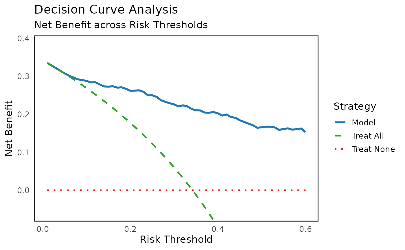
This function evaluates the clinical utility of the confounder-adjusted risk model by quantifying net benefit across a range of decision thresholds and comparing against two reference strategies: treating all patients or treating none.
Usage
dca_analysis(
  adjust_result,
  outcome,
  thresholds = seq(0.01, 0.6, by = 0.01),
  risk_col = "adjusted_risk",
  ylim_lower = NULL
)
Arguments
- adjust_result
Output list from
adjust_score(), containing the augmented dataset with risk scores and outcome.- outcome
Character, name of binary disease outcome column (0/1).
- thresholds
Numeric vector of risk thresholds (default = 0.01 to 0.60 by 0.01).
- risk_col
Character, name of the risk score column to use (default = "adjusted_risk"). Allows generalisation beyond the default adjusted risk output.
- ylim_lower
Numeric, lower bound for the y-axis in the decision curve plot. If
NULL(default), the bound is computed dynamically asmin(NB_model, -0.05, na.rm = TRUE) - 0.01.
Value
A list with:
data: Data frame of net benefit values for each strategy across thresholds.plot: ggplot object showing the decision curve.
Details
Concept
DCA is a method to assess whether a predictive model improves clinical decision-making compared to default strategies.
Net benefit (NB) balances true positives against false positives, weighted by the risk threshold: $$NB(t) = \frac{TP(t)}{N} - \frac{FP(t)}{N} \cdot \frac{t}{1-t}$$ where \(TP(t)\) and \(FP(t)\) are counts at threshold \(t\), and \(N\) is the total sample size.
Interpretation: The model is clinically useful at thresholds where $$NB(model) > \max(NB(treat\ all), NB(treat\ none))$$.
Implementation
Input: adjusted risk scores from
adjust_score()and true disease labels.Thresholds: defaults to 0.01-0.60 in steps of 0.01 (\(1\%\) to \(60\%\) risk).
Strategies compared:
Model: net benefit using adjusted risk predictions.
Treat All: assume all subjects are positive.
Treat None: assume all subjects are negative.
Output: a data frame of net benefit values across thresholds and a ggplot decision curve showing the three strategies.
Examples
n <- 500
set.seed(123)

# outcome
DISEASE <- rbinom(n, 1, 0.35)

# biomarker depends on disease
PTAU <- rnorm(n, mean = 25 + 10 * DISEASE, sd = 8)

# confounders (optional noise)
AGE <- round(rnorm(n, 73, 7))
SEX <- sample(c(0, 1), n, replace = TRUE)
BMI <- rnorm(n, 25, 4)
HTN <- rbinom(n, 1, 0.3)
DM <- rbinom(n, 1, 0.2)

df <- data.frame(PTAU, AGE, SEX, BMI, HTN, DM, DISEASE)
res <- adjust_score(df,
biomarker = "PTAU",
outcome = "DISEASE",
confounders = c("AGE","SEX","BMI","HTN","DM"))
#> number of iterations= 704
#> Setting levels: control = 0, case = 1
#> Setting direction: controls < cases

dca_out <- dca_analysis(res, outcome = "DISEASE")
head(dca_out$data)
#>   Threshold  NB_model    NB_all NB_none
#> 1      0.01 0.3353535 0.3353535       0
#> 2      0.02 0.3285714 0.3285714       0
#> 3      0.03 0.3216495 0.3216495       0
#> 4      0.04 0.3145833 0.3145833       0
#> 5      0.05 0.3076842 0.3073684       0
#> 6      0.06 0.3016596 0.3000000       0
print(dca_out$plot)